
Radiative heat loss from PV systems
Our latest white paper examines how radiative heat loss to the sky affects PV module temperatures and yield forecasts. We found that ignoring sky temperature in thermal models can introduce up to ±0.5% uncertainty in annual yield predictions.

· Keith McIntosh · 8 min read
See the full white paper here.
A nighttime puzzle
Several years ago, we were asked to analyse data from a PV test facility. It was the first time we’d received nighttime data and we were surprised to see that after sunset, the modules became colder than the ambient air.
Module and ambient temperatures over a 24 hour period 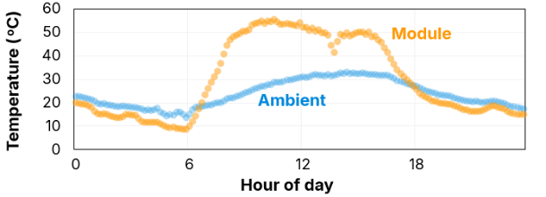
Now, since the conventional temperature model used by the PV industry — the Faiman model — predicts that module temperature at night must equal the ambient temperature, we hastily concluded that there was a bias in the measurements. ‘Your thermocouples have a negative offset,’ we told the facility, and we adjusted the module temperature accordingly.
We’re probably not the first to have embarrassed ourselves by making this wrong conclusion, and we’re probably not the first to have had a ‘eureka’ moment a few weeks later, and then to find that this oddity had been explained long ago.
The nighttime offset was, in fact, genuine. It was caused by radiative cooling. And as good ol’ Duffie and Beckman explain, a solar panel absorbs heat from the ambient air and radiates it into the cold night sky. This flow of heat means that the module temperature must lie somewhere between the air temperature and the sky temperature.
Why is this observation relevant to PV power plants? Well, it’s a simple illustration of how the Faiman model does not accurately account for radiative heat loss to the sky.
Moreover, it leads to more important questions:
Does radiative heat loss introduce a discrepancy between the Faiman model and reality during the daytime? And if so, is the discrepancy large enough to matter for yield forecasts? And if so, can we use thermal physics to improve our forecasts?
These questions are examined in our latest white paper called “Radiative heat loss from PV systems”.
This blog post describes the key takeaways from our study. Refer to the white paper for the gory details.
Radiation to the sky: A major contributor to the heat loss
Solar panels radiate 30% to 60% of their heat to the sky during the day. If the sky is cold, the panels radiate more heat, helping them to operate at a lower temperature and hence to generate more electricity.
The figure below illustrates the scale of the radiative loss for a single-axis tracker (SAT) near Denver. It explains what happened to the solar energy that fell on the PV modules over the course of two days, where the first day was sunny and the second day was also sunny until dark clouds rolled in and spoiled the afternoon. The figure shows that about 20% of the solar energy was converted into electricity (orange area), and the remainder was emitted as heat (blue area). Of that heat, about a third was radiated to the sky around midday, and an even higher fraction was radiated at the shoulders of the day and at times of thick cloud.
The figure also shows that after sunset the modules absorbed heat from the air and radiated it into the night sky. Even at night we can study the behaviour of PV modules!
Energy flow diagram 
Accounting for radiative heat loss in yield forecasts
Most yield forecasts apply the simple Faiman thermal model, which bundles all thermal losses into a single equation and assumes them to depend on the difference between the module temperature and the ambient temperature (Tmod – Tamb).
While simple equations have their advantages, it is more accurate to say that radiative heat loss depends on (Tmod – Tsky), where Tsky is the sky temperature. (See the white paper for the complete equations.)
We can see in the figure below that the Faiman model must introduce error. The figure plots Tsky vs Tamb for every hour of the year at Roskilde, which is coastal and wet, and at Albuquerque, which is inland and dry. It shows that for the same Tamb, the sky in Albuquerque is 10–20 °C colder than in Roskilde. Consequently, on a day with the same irradiance and Tamb, we expect more radiative cooling — and hence a higher yield — in Albuquerque than Roskilde. And yet the simple approach to radiative loss would not have predicted any difference at all.
Our white paper calculates the error in yield introduced by the Faiman approach at several sites. It also describes how the error can be mitigated with a more realistic radiative model.
Sky vs ambient temperature comparison 
Experimental validation
Before evaluating the yield, we tested the applicability of a realistic radiative model at five experimental test sites by comparing measured and simulated module temperatures. The simulations used one of three thermal models:
| Model | Inputs | Approach to radiative heat loss |
|---|---|---|
| M1 | Industry standard* | Simple |
| M2 | Calibrated | Simple |
| M3 | Calibrated | Realistic |
*Uc = 29, Uv = 0
Importantly, the realistic model for radiative heat loss did not introduce any additional free variables. It simply distinguished between the heat lost to the ambient and the heat lost to the sky, and it loaded Tsky from satellite data.
The figure below plots the results. It shows that the realistic approach gave a superior prediction of module temperature for four of the five sites. In the best case, the root-mean-square error (RMSE) in module temperature was reduced from 3.0°C to 1.8°C, just by introducing the realistic model for radiative loss (compare M3 to M2).
These results demonstrate that a realistic thermal model — with no additional free parameters — can increase the accuracy of yield forecasts.
Model validation results 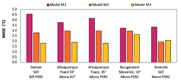
Error in yield forecasts due to radiative losses
Most yield programs, including PVsyst, apply the simple Faiman thermal model. This involves setting one or two ‘U-values’ that govern the heat lost to the ambient, and that are assumed to be constant at all times of year.
As we’ve discussed, however, radiative heat loss actually depends on Tsky, which changes (relative to Tamb) from day to day, from season to season, and from site to site. This means that the radiative component to the U-value must also be continually changing, and hence the assumption the U-values are constant introduces error.
How much error?
The figure below plots the error in the daily yield for a particular SAT configuration. The error has been calculated after calibrating its U-values to give the best fit to a three-week testing period at the Denver test facility. Thus, the calculated error is as low as possible and accounts only for changes in radiative heat loss.
The figure shows how the error varies from site to site, and how it becomes more negative when humidity and diffuse fraction (related to cloud cover) decrease. The error for the cold, dry sites of Denver, Albuquerque and Chajnantor (in the Atacama Desert) are about 0.6–1.0% different to the error in the warm, humid site of Singapore. And, in Albuquerque, the error on a very dry day is about 1% different to the error on a humid day.
We also found that seasonal changes in error are typically 0.4% but can be anywhere between 0.1% and 1.1% depending on the site and configuration. (The error is larger for fixed-tilt systems than for SATs.)
Yield forecast error analysis 
Improving accuracy with a realistic radiative model
We have seen that the simple approach used in most yield software introduces uncertainty by assuming constant U-values. We conclude that, by itself, this assumption introduces up to ±0.5% uncertainty in the annual yield, and an additional ±0.5% into the daily yield.
Errors of this magnitude are, in many cases, not negligible. If an inaccurate prediction of the radiative losses caused the yield to be under or overestimated by 0.5% or 1%, it could be the difference between a pass or fail on a commissioning test.
Fortunately, much of this error can be mitigated by applying the more realistic equations for radiative heat loss. These equations have been implemented in SunSolve Yield. That’s not to say that the radiative and non-radiative models cannot be refined and validated further, and we encourage PV researchers to continue studying the thermal behaviour of PV systems.
Download the white paper to learn more about radiative heat loss in PV systems and how it affects yield predictions.
Beyond temperature modeling: A physics-first approach to PV simulation
The improvements to thermal modeling described in this paper represent just one area where SunSolve has advanced beyond the status quo. Our mission is to deliver research-grade simulation tools for the solar industry by applying rigorous physics-based modeling at every step - optical, thermal, and electrical.
While many yield modeling tools focus primarily on annual energy estimates, we believe that accurate modeling begins with getting the fundamentals right at each individual timestep. Only by establishing this solid foundation of physics-based accuracy can we deliver truly reliable predictions across an entire year of operation.
Whether it’s implementing realistic radiative heat transfer, accounting for complex optical interactions, or modeling electrical behavior with precision, SunSolve is committed to advancing the science behind PV simulation - one step at a time.
Get Started Today
Ready to experience research-grade PV modeling? Contact us to discover how SunSolve’s physics-first approach can transform your performance forecasts.
Acknowledgments
This work was supported by funding from the Australian Renewable Energy Agency (ARENA). The views expressed herein are not necessarily the views of the Australian Government, and the Australian Government does not accept responsibility for any information or advice contained herein.