
Understanding cell-to-module loss: how simulation helps close the gap
Cell-to-module loss (CTM) sits at the intersection of cell and module engineering. As cell performance approaches practical limits, the challenge is how much of that value survives into the finished module. This article introduces CTM and shows how simulation tools are being used to understand, predict, and optimise the cell-to-module transition.
· Mal Abbott · research · 17 min read
Cell-to-module (CTM) loss is a critical metric when developing a solar product. However, it is much less common to see it reported. What tends to grab the headlines is the cell efficiency, module efficiency and module power. That is not to say the industry does not care about it. Quite the opposite.
Over the years we have had many engagements with teams from industry wanting to understand, quantify and optimise this metric. Interestingly this work has tended to come in waves. It peaks when new cell architectures are emerging, or when new companies are ramping up production. We are currently in one of those peaks. Cell sizes are changing, with different wafer cutting schemes being explored (i.e. the so called third-cut and quarter-cut modules). The all-back-contact solar cell is once again trying to assert itself as a viable cell option. The HJT and TOPCon solar cells continue to push the bounds on what anyone thought was an upper limit to 1-sun conversion efficiency for a mass produced cell. And perovskite tandem cells are pushing towards commercialisation. As a result we are again seeing a lot of requests to understand and optimise CTM. This post is for anyone coming into this space fresh and wanting to get up to speed on the fundamentals — and for those already deep in it who could use a simulation tool to move faster.
The first thing I would say about CTM, is that measuring it can be difficult. It requires an IV test of both the cell and module. These tests already have significant uncertainty in them. Adding to the challenge is the fact that IV testers tend to not even be in the same building (sometimes not even the same city!). Beyond that is another business related challenge. Most PV companies I have worked with tend to have a divide between the cell team and the module team. That makes some sense from a technical perspective, but it means that CTM lands right between the two teams. Engineering changes on either side of this invisible wall can impact CTM. When that happens, it is very useful to have an established protocol to not just measure the absolute CTM, but to break it down into its components (dare I say, to point the finger at the culprit). An example of that is shown in the waterfall chart below. It was produced with SunSolve simulations, based on an experimental procedure developed by Dr Haedrich from Fraunhofer ISE (more on that later).
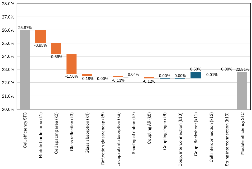 Figure 1: Example CTM waterfall chart for an all-back-contact cell architecture, showing the individual loss and gain factors from cell to module. Produced using SunSolve.
The waterfall chart gives us 13 ‘k’ factors that quantify the losses and gains associated with the change in output power as we move from an STC test of a solar cell under air, into a fully encapsulated module. The CTM value is derived from the first and the last column. Everything in between tells us how we got there and more importantly how we can improve module power. Creating this chart experimentally is possible, but it requires a lot of work and limits the options in terms of variations in inputs. With a physics-based solver like SunSolve we can predict the optical and electrical impact of this encapsulation process. We ground the result in measurement, then allow the user to rapidly iterate on the inputs to identify a path to improvement.
The next few sections of this post will introduce CTM and describe some of the fundamentals. If you are only interested in how to create the chart you see above then feel free to skip ahead to the section “How to use SunSolve to calculate CTM?”.
What is CTM?
CTM stands for Cell-To-Module. It is often used to either express a ‘CTM ratio’ or ‘CTM loss’. These are defined as seen below, most commonly using cell and module STC power measurements.
When I first studied photovoltaics (back in the early 2000s) it was very common to always talk about CTM loss. Back then it was typical for that loss to be anywhere from 2 – 8%. However as engineers got better at integrating cells into modules this ‘loss’ was greatly reduced and in some cases even turned into a gain. In recent years it is common to use CTM ratio as the general term, and then talk about losses and gains when breaking down the contributors.
The equations above compare power, which is typically what a manufacturer sells. However, it is also interesting to compare efficiency. Now we are normalising for areas which may be more relevant to the system developers. The equations are similar, both cells and modules are tested with the same irradiation, so we just need to include the area.
The definition of the cell area is clear. The area of the module however can have some variation. Is it an apertured area? Do we want to include the area of frames in CTM value we report? That is somewhat up to the engineer.
When CTM is defined using efficiency rather than power, the result depends not only on electrical and optical cell-to-module effects, but also on the chosen definition of module area, such as aperture area, laminate area, or total framed area.
At the end of the day, like all these metrics, choose what gives you the insight you want to report on (and/or improve). Power-based CTM captures the effect of module assembly on power, whereas efficiency-based CTM also includes the area penalty associated with gaps, borders, and potentially the chosen frame or module area definition.
CTM is not a new concern
When I sat down to write this blog post my mind traveled back to an event in 2016 (almost exactly 10 years ago). It was the very first ever PVModuleTech conference and we had been offered a speaking slot. It turned out to be a fantastic event with a room packed full of the who’s-who of the PV world. At PV Lighthouse we had released an early version of SunSolve and wanted to show the world how it could be used to understand cell to module loss. At that time there was great work being done at research institutes to help understand the problem. The team at Fraunhofer ISE played a key role in developing measurement and analysis techniques to provide insights into CTM. One outcome of that work was the paper I referred to earlier, produced by Dr Haedrich.1 It provided a detailed process for quantifying 13 separate loss and gain factors. The experimentation required was tricky, but it worked well. All of that work is still very much relevant today. The cells may have improved, but the fundamentals of module encapsulation remain unchanged.
Before PVModuleTech I spent hours searching the internet to collect up a large number of cell and module data sheets (I must have had more time to prepare for conference talks back then!). The idea was to quantify the current state of the industry. It is always hard to gauge this from scientific articles and press releases where we often see champion results. The data sheet is very much where the rubber hits the road when it comes to actual panels being sold. Below is the first pair of plots I presented. They are scatter plots of cell and module power separated by the old division of polycrystalline versus monocrystalline. In the monocrystalline category an exciting new cell architecture PERC had just started to appear and compete with the then ‘standard’ Al BSF cells. The average of all data points is marked in orange, and the difference between any two similar groups we interpret as the average cell to module loss in the industry.
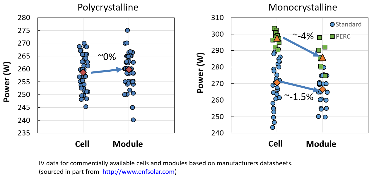 Figure 2: Scatter plots of cell and module power separated by polycrystalline versus monocrystalline technologies (2016 data).
The first thing we noticed was that the average CTM for polycrystalline-based technologies was 0%! Job done right? The monocrystalline still had a little way to go with losses of 1.5% for standard cells and 4% for the new kid on the block. Now look at how those same data sets look when we plot the efficiency:
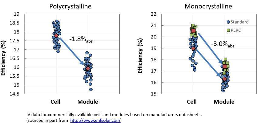 Figure 3: Scatter plots of cell and module efficiency separated by polycrystalline versus monocrystalline technologies (2016 data).
Yikes, this does not look like job done. A 1-sun efficiency drop of around 2% absolute for the polycrystalline and around 3% absolute for both cell types on monocrystalline. Here we are seeing the key difference between CTM based on power and CTM based on efficiency. When you build a module, you add extra area. The white space around the cells reflects some of the light onto the cells, increasing the power. However, it is never as efficient at converting the incident light into power as an actual active area of the solar cell. The frames, if included in the efficiency calculation, add nothing at all.
Before we move on, let’s just take a little look at fundamentally what was driving the CTM. One way to do this with measured data is to break down the earlier comparison into the key metrics of Isc, FF and Voc. The Voc did not change at all, so I’ve not plotted it here. More interesting are the Isc and FF.
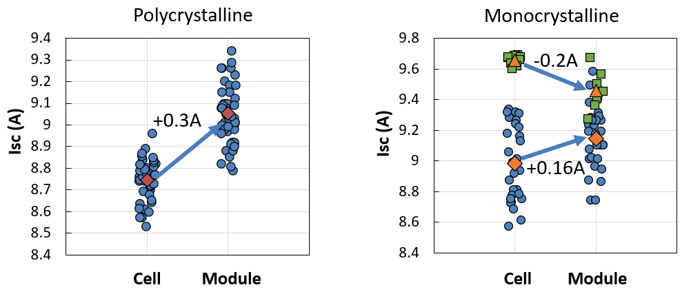 Figure 4: Breakdown of CTM effects into Isc for polycrystalline and monocrystalline technologies (2016 data).
The Isc increases for the polycrystalline and standard BSF cells. This occurs despite the addition of glass reflection and absorbing materials like EVA. One reason is that there are optical gains to be had when we encapsulate our cells. Light reflected from the front side texture and metal grid may be internally trapped by the glass, thus reducing the loss and increasing the current. That was particularly effective for the polycrystalline where the front texture was not as good as the upright random pyramids used on monocrystalline devices.
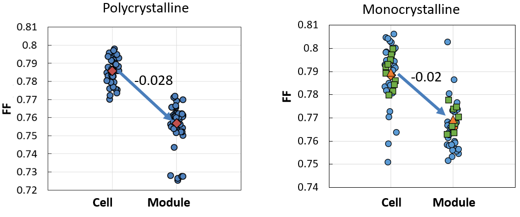 Figure 5: Breakdown of CTM effects into FF for polycrystalline and monocrystalline technologies (2016 data).
The FF decreases in all cases. When we interconnect cells, we use a conducting ribbon which must carry the current between the cells. This adds a more resistive path compared to IV probes used during cell testing (which extract the current directly from the busbar). You can reduce this loss by adding more ribbons — or by making those ribbons larger — however that leads to optical losses (and possibly cost increases).
All these effects — optical and electrical — can be predicted with simulation tools. SunSolve is particularly suited to this task. It models optical materials via their wavelength-dependent complex refractive index and employs highly detailed ray tracing, which models the propagation of light through the many layers within a PV module. It implements scattering models which are critical at the surface of fingers and in the white space that surrounds the cells. On the electrical side, SunSolve includes an analytical grid resistance model that calculates the series resistance, connecting the electrical resistive losses to the optical losses/gains within the software.
How to use SunSolve to calculate CTM?
Within a single SunSolve simulation the user can solve the 1-sun STC output power and get a detailed breakdown of the optical losses. To calculate the CTM we need to run two simulations and compare the results. Initially what is required is a baseline model for the solar cell and a baseline model for the module. This is always the first step we go through with new users of SunSolve. We need to build up models that match what they are producing with their best known method. It is an iterative process, and is too detailed to cover here. It does not need to take long however, as SunSolve has many materials in its database that already provide a good starting point.
From these two simulations we can determine the ratio of output power, hence our CTM. Engineers can already then experiment with design changes and measure the impact on CTM. This is useful, but it does not provide us with the nice waterfall breakdown we saw at the start of the article. Producing that requires a little more simulation effort.
Next, we provide our users with detailed instructions on how to simulate the test structures reported in the paper by Dr Haedrich.1 It turns out that we need seven simulations (including the two baseline sims) to extract 12 of the 13 ‘k’ factors from the paper. The final factor relates to the resistive losses incurred by connecting the cell strings to the module terminals. Those losses are not currently calculated in SunSolve and need to be added manually.
In some cases it is possible within SunSolve to simply reproduce the experimental test structure. For example, the determination of k[8, 9, 10] requires the following:
For this we take our baseline solar cell simulation, then add the ribbons and a layer of EVA on top. Note that the experiment calls for a ‘high absorptive black back sheet’. This is required to minimise any Isc signal coming from the cell surrounds and focus in on what is happening at the cell surface. Here we have an advantage with simulation, we can remove that area from the simulation, or we can set the absorber to be perfectly black.
In other cases the simulation approach makes it much easier to extract the factors. To determine coupling gains from cell surroundings k[11] the paper requires an engineer to make a one-cell laminated mini-module, vary the reflective surround width with a mask, measure short-circuit current, fit the trend, and then translate that result to the real module’s cell spacing and cell shape. In SunSolve we can just turn off the rear reflector. At this point an engineer may well ask: how is that SunSolve approach going to reflect reality without the use of an experimental measurement? The answer is that the result is based on the approach applied to create the baseline module. If we selected a generic backsheet material from the default settings in SunSolve then that is the result we will see for k[11]. However, we will usually refine the inputs to our baseline modules using measurements. In that case we want test structures that are as simple as possible. For backsheets you can measure them under air, then convert them into an encapsulated value. Now we are at risk of getting into the weeds here so we won’t keep spiralling deeper. I think the point is that we have done all this before and can help navigate our users through it all.
The full set of factors is summarised in the figure below, reproduced from the original paper. A detailed breakdown of each factor — and how to extract it using SunSolve — can be found in the appendix.
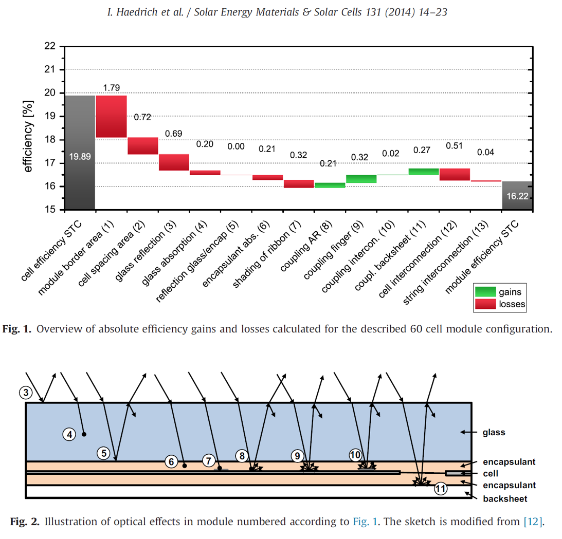 Figure 6: Breakdown of CTM loss and gain factors based on the Haedrich methodology.
Closing the gap
There have been many innovations since Dr Haedrich first wrote her paper in 2014. It was never written with all-back-contact cells or bifacial modules in mind. The original approach can be adapted to these new architectures, and we have already done so with several of our industry partners. The use of simulation also unlocks the possibility to add some new factors. For example the original paper neglects the cell-to-cell mismatch loss that occurs when cells are interconnected into strings. This is easily added in when using SunSolve. Looking towards the future, the full spectral capabilities of SunSolve make it ideal for simulation of tandem devices. In that space optimisation of the cell-to-module losses will be critical to maintain the high cell efficiencies. SunSolve calculates the mismatch loss between vertically stacked sub-cells, this could be added in and CTM calculated for different spectral conditions.
The physics that drives CTM is complex: optical, electrical, and geometrical effects all interact, and they change depending on the cell architecture, the encapsulation materials, and the module layout. This complexity is why simulation becomes so useful. It allows us to replace painstaking experimental iteration with fast, accurate modelling complemented by simplified experimentation.
If you would like to learn more about CTM, or if you are ready to dive in and start using SunSolve to calculate it, then please contact us.
Appendix: CTM factors and SunSolve simulations
For reference, the tables below summarise all 13 ‘k’ factors from the Haedrich methodology, the SunSolve simulations used to extract them, and how each factor is obtained.
SunSolve simulations
| Sim | Model | Main metrics extracted |
|---|---|---|
| 0 | Baseline solar cell | Cell power and/or cell efficiency (P0) |
| 1 | Full baseline module | Module power, module Isc, spectral front reflection, spectral glass absorption, spectral front encapsulant absorption |
| 2 | Full module with no optical ribbon loss | Module power and/or module Isc for ribbon-loss comparison |
| 3 | Full module with absorbing rear white-space regions | Module power, module Isc, or preferably average cell current for rear-coupling comparison |
| 4 | Solar cell with ribbons | Cell current/power in the uncoupled case |
| 5 | Solar cell with ribbons and EVA | Cell current/power in the encapsulated case |
| 6 | Glass–encapsulant reflection test structure | Spectral reflection at the internal glass–encapsulant interface |
The 13 k-factors
| Factor | Name | Type | Description | SunSolve approach |
|---|---|---|---|---|
| k1 | Module border area | Geometric loss | Inactive area around the outside of the cell matrix increases module area and reduces efficiency. | Analytical calculation from module and cell matrix areas. No simulation needed. |
| k2 | Cell spacing area | Geometric loss | Inactive area between cells increases total area and reduces efficiency. | Analytical calculation from total cell area and module area. No simulation needed. |
| k3 | Glass reflection | Optical loss | Reflection at the air–glass interface. | From Sim 1: spectrally weight front-surface reflection against cell response. |
| k4 | Glass absorption | Optical loss | Absorption in the front glass. | From Sim 1: spectrally weight glass absorption using cell response. |
| k5 | Reflection glass/encapsulant | Optical loss | Reflection at the glass–encapsulant interface. Usually very small. | From Sim 6. Often approximated as 1 and skipped. |
| k6 | Encapsulant absorption | Optical loss | Absorption in the front encapsulant only. | From Sim 1: spectrally weight front EVA absorption using cell response. |
| k7 | Shading of ribbon | Optical loss | Optical loss from interconnection above the cell. | Compare Sim 1 with Sim 2; derive factor from power difference. |
| k8 | Coupling AR | Optical gain | Recapture of light reflected from non-metal cell surface via internal reflection in the encapsulation stack. | Compare Sim 4 with Sim 5 to isolate encapsulation-induced recapture. |
| k9 | Coupling finger | Optical gain | Recapture of light reflected from fingers, including changed metal optics under encapsulation. | Effective width ratio / metallisation correction from additional runs or a default technology value. |
| k10 | Coupling interconnection | Optical gain | Recapture of light reflected from ribbons / interconnections. | Effective width ratio / interconnection correction from extra runs, or a default technology value. |
| k11 | Coupling backsheet | Optical gain | Light reflected from surrounding white space and collected by the cell, including losses in that optical path. | Compare Sim 1 with Sim 3. Use average cell current, not string-limited current. |
| k12 | Cell interconnection | Electrical loss | Resistive loss in cell-to-cell ribbons / interconnects. | Compare baseline module power with interconnection resistance set to zero. |
| k13 | String interconnection | Electrical loss | Resistive loss outside cell interconnects (junction box, string connections). | Not simulated in SunSolve; add from measurement or electrical assumptions. |
1 I. Haedrich, U. Eitner, M. Wiese, H. Wirth, “Unified methodology for determining CTM ratios: Systematic prediction of module power”, Solar Energy Materials and Solar Cells, Volume 131, 2014, Pages 14-23, ISSN 0927-0248