
Calculating the bifacial gain of AgriPV systems with SunSolve and PVsyst
This post explores how to predict the bifacial gain of AgriPV systems, which can vary from 2% to 50% depending on system design and conditions. We describe SunSolve's ray-tracing method, PVsyst's industry-standard approach, and how they can be used together.
· Keith McIntosh · research · 9 min read
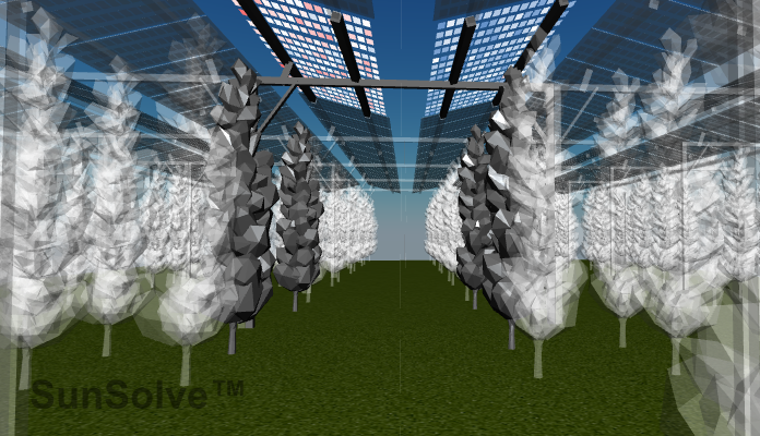
AgriPV systems must allow plenty of sunlight to fall upon the crops below. The modules are therefore widely spaced and sometimes semitransparent, e.g., see Figure 1(a), which is quite different to conventional systems. This design permits a good fraction of that sunlight to reflect from the ground and crops onto the rear side of the modules, providing a second opportunity for AgriPV modules to convert sunlight into electricity. That’s why AgriPV systems almost always contain bifacial modules.
And so, as interest in AgriPV grows, we’re hearing one question more and more frequently:
How can I predict the bifacial gain from my AgriPV system?
This post describes a couple of approaches to answering that question.
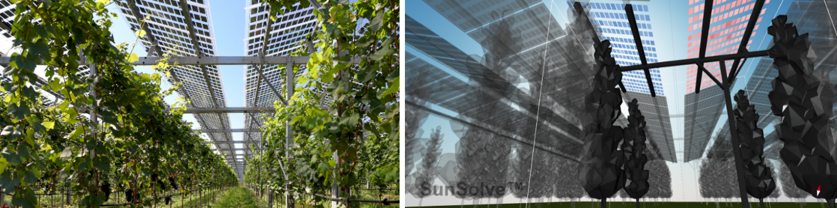 Figure 1: (left) Actual and (right) simulated view of a bifacial waves AgriPV system with semitransparent modules.
Is there a typical bifacial gain for AgriPV?
Since the bifacial gain contributes significantly to the electrical yield of AgriPV systems, it is important for engineers to predict how the gain is affected by module layouts, orientations, and structural supports.
Unfortunately, there is no single estimate for the bifacial gain in AgriPV systems. The variety of AgriPV designs is too great — with many systems being customised to the available land or the particular crop — and moreover, the gain changes throughout the day and year.
For example, the annual gain for the system of Figure 1 is computed to be 6%, but the gain at any point in time is as low as 4.3% at midday on a clear summer day, or up to 48% when the sun is near the horizon. To illustrate this variability, Figure 2 plots the gain at every hour of the year, showing how (a) the gain is lowest when the sun is high in the sky, increasing slowly as the sun descends and then rapidly once the sun is within 10° or 15° of the horizon; and (b) the gain is lowest under clear skies, increasing as the sky becomes cloudier.
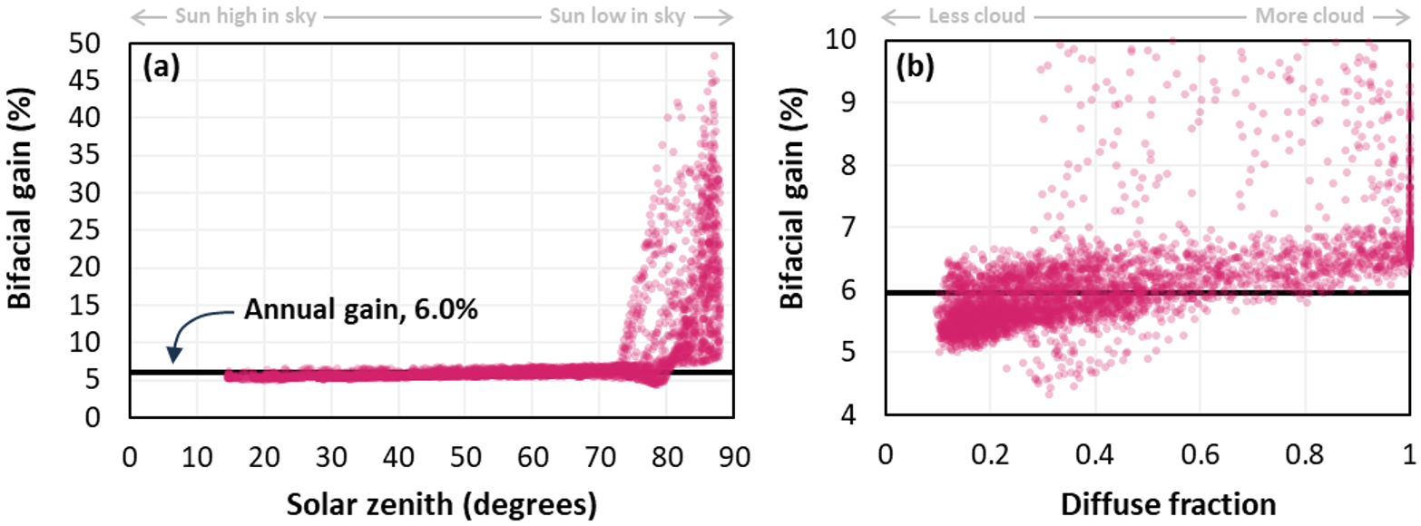 Figure 2: Bifacial gain of the system in Figure 1 plotted against (a) solar zenith and (b) diffuse fraction. Symbols plot gain at each hour of the year; line plots annual gain.
The values in Figure 2 are specific to the wave-type AgriPV system in Figure 1. In systems whose modules are more closely spaced, or whose modules are less transparent, or whose crops are more absorbing, or whose structural supports are more obtrusive, the gain would be significantly smaller. And, of course, the inverse is also true.
Furthermore, AgriPV systems can sometimes use vertical modules (Figure 3), or trackers, or various orientations of fixed systems, for which the annual gain can vary from 2% to 50%.
So, is there a quick and reliable method to estimate the bifacial gain in AgriPV systems?
We describe two possible approaches: SunSolve and PVsyst.
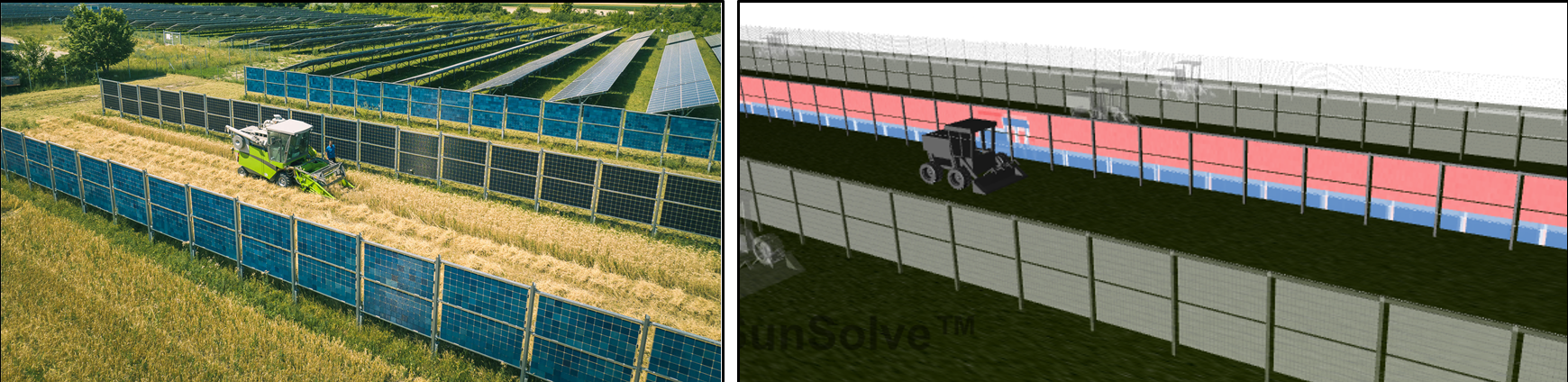 Figure 3: (a) Actual and (b) simulated view of a vertical bifacial AgriPV system.
SunSolve
SunSolve Yield provides a quick and intuitive way to determine the bifacial gain of an AgriPV system.
To create a bifacial AgriPV system in SunSolve, one defines the physical dimensions of the system by setting the orientation and layout of the east- and west-facing modules, by loading the system’s structural supports from CAD models, by selecting either opaque or semitransparent modules, by stringing the east- and west-facing modules to the inverter and, if desired, by adding crops below the modules.
As shown in Figure 1(b), SunSolve contains a 3D visualisation of the simulated system, which helps confirm whether the virtual system has been created correctly.
SunSolve then uses ray tracing to simulate the system optics, calculating the front and rear irradiance on each cell before solving the electrical circuits of the modules and strings. The annual yield is solved in 1–10 minutes, where the duration depends on the optical complexity of the module and whether the timesteps are 5, 15 or 60 minutes. The calculations include spectral and thermal effects, as well as the electrical mismatch arising from non-uniform irradiance.
Finally, to compute the bifacial gain, two simulations are run in parallel: (i) the baseline simulation, and (ii) a modified simulation in which light is prevented from entering the rear of the module. The relative difference between these simulations is the bifacial gain.
PVsyst
Another way to model the bifacial gain is to use PVsyst, the industry standard software for system modelling.
At the time of writing, however, this necessitates a complicated procedure when simulating wave systems. Although PVsyst contains the option to simulate ‘domes’ (a waves system), it does not permit them to be bifacial. Consequently, one must create two separate ‘infinite-shed’ systems—one for the east-facing and another for the west-facing modules—and select the bifacial option for both.
PVsyst’s optical model then computes the irradiance on the rear of the module as if (i) there are no lateral gaps between modules, (ii) the modules are opaque, and (iii) the neighbouring rows of modules are exclusively of the same type of system. Thus, to simulate the east–west waves structure of Figure 4(a), PVsyst simulates the rear optics of the east-facing modules as if the west-facing modules were not present as shown in Figure 4(b), and the equivalent case for the west-facing. Having calculated this ‘ideal’ case with a view-factor approach, PVsyst then modifies the rear irradiance with two optical factors, the ‘structure shading factor’ fS and the ‘shed transparent factor’ fT, and modifies the resulting output power by a rear-side ‘mismatch loss factor’ fMR.
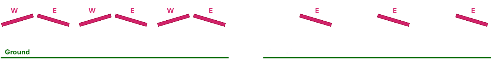 Figure 4: (a) East- and west-facing modules and (b) just the east-facing modules.
This approach therefore requires the user to enter values for fS, fT and fMR, where:
- fS accounts for rear-side shading by structural supports and any crops, as well shading by the missing neighbouring row of modules (e.g., the missing west-facing modules when simulating an east-facing row);
- fT accounts for additional rear irradiance arising from either light passing between lateral gaps between modules or passing through semi-transparent modules; and
- fMR accounts for electrical mismatch loss arising from non-uniform irradiance and the rear.
None of these inputs are simple to calculate from simple geometric principles, nor can they be measured without a complicated experimental setup that replicates the system.
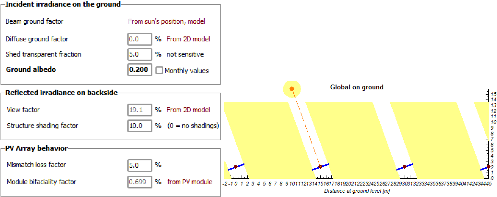 Figure 5: Screenshots of PVsyst’s bifacial system interface: (left) ‘Bifacial system definition’ screen (right) ‘Unlimited Trackers 2D Model’
SunSolve and PVsyst combined
PVsyst constitutes the industry standard for yield forecasting, and its reports are readily interpreted and trusted. It’s therefore important that the industry has a well-defined procedure for determining fS, fT and fMR for AgriPV systems — and any other bifacial system.
The common way to determine fS, fT and fMR is with programs that combine ray tracing and SPICE, such as SunSolve.
The procedure involves creating the system in SunSolve that best represents the actual system. In that case, fS, fT and fMR are zero; i.e., no corrections are applied because the simulation already accounts for shading, transmission and mismatch. One then modifies the SunSolve inputs so that the simulations increasingly mimic the ‘ideal’ system simulated by PVsyst, which has no supports, spacing, transparency or mismatch. After each simulation, one can determine another correction factor. For example, fS is determined by comparing the solution when structural components are excluded to that when they are included.
The procedure to determine those factors is described for SAT and fixed-tilt systems here. (It has been automated for SunSolve users.) This procedure will also work for vertical PV systems, provided the PVsyst simulation treats the east- and west-facing rows as two separate infinite-shed systems where the optical pitch is set to the distance between the east- and west-facing rows.
But the procedure will not yet work for wave-type systems. A new procedure is required where the non-baseline simulations exclude the opposite-facing modules to mimic PVsyst.
Figure 6 plots fS, fT and fMR for the wave system of Figure 1. The lines represent the energy-weighted annual average, as would be entered into PVsyst. The symbols show the energy-weighted daily values, which have a seasonal dependence due to changing solar position and weather. We describe the reasons for these and other trends in our paper “Bifacial factors of Agri-PV systems” presented at the EU PVSEC in 2025. Contact us for a pre-print of the paper.
 Figure 6: Daily (symbols) and annual (lines) fT, fS and fMR for the waves systems of Figure 1 with east-facing rows in orange and west-facing rows in red. These values of fS and fT differ from what one would expect for shading and transmission factors because they are determined for the double infinite-shed approach proposed for PVsyst.
Conclusion
SunSolve Yield provides an intuitive and sophisticated approach to solving the gain. It’s also possible to use PVsyst to solve the gain, but this requires the user to enter three bifacial factors determined by programs like SunSolve.
We hope that by using simulation tools such as these, and combining them with accurate experimentation, the PV industry can establish validated procedures for forecasting the energy yield of AgriPV systems.
Interested in simulating your AgriPV system?